Understanding OpenCV - Code Snippets
I made a jump directly to Computer Vision by using Deep Learning, mostly using CNNs & Keras. CNN & Keras are like Adam West’s Batman & Burt Ward’s Robin, much simpler & fun days of the bat vigilante.
Source: The Mary Sue
But with a lot of image pre-processing (apart from Keras’ own functions) crucial to the final output, I searched for a good library to do it. skimage is a great library for doing image pre-processing. It packs enough to get you started, but the most widely used is OpenCV.
OpenCV has a bit of steep learning curve, but once you get used to it there’s no feeling like any other. While preparing this notebook, I never intended it to be a blogpost. Things started off with creating snippets off the official library & with inputs from blogposts by PyImageSearch which is frankly the most comprehensive blog for Computer Vision. Let’s dive into the actual notebook.
Downloading the image
!curl "https://raw.githubusercontent.com/pratos/pratos.github.io/master/images/screenshot1.png" > screeshot.png
  % Total    % Received % Xferd  Average Speed   Time    Time     Time  Current
                                 Dload  Upload   Total   Spent    Left  Speed
100 74844  100 74844    0     0  73184      0  0:00:01  0:00:01 --:--:-- 78866
!ls
Amazon Kaggle EDA.ipynb			      Pre Processing Notebook.ipynb
Image Processing using OpenCV - Part 1.ipynb  screeshot.png
Import the image through OpenCV
%matplotlib inline
import matplotlib.pyplot as plt
import signal
import numpy as np
import cv2
- Open an image using cv2.imread()
- Import a color image: cv2.IMREAD_COLOR (arg = 1)
- Import a color image: cv2.IMREAD_GREYSCALE (arg = 0)
- Import a color image: cv2.IMREAD_UNCHANGED (arg = -1)
screen_img = cv2.imread('./screeshot.png', 1)
plt.imshow(screen_img)
plt.xticks([]), plt.yticks([])  # to hide tick values on X and Y axis
plt.show()

Drawing shapes on an image
# Create a black image
img = np.zeros((512,512,3), np.uint8)
# Draw a diagonal white line with thickness of 6 px
cv2.line(img, (0,0),(511,511),(255,255,255),6)
array([[[255, 255, 255],
        [255, 255, 255],
        [255, 255, 255],
        ...,
        [  0,   0,   0],
        [  0,   0,   0],
        [  0,   0,   0]],

       [[255, 255, 255],
        [255, 255, 255],
        [255, 255, 255],
        ...,
        [  0,   0,   0],
        [  0,   0,   0],
        [  0,   0,   0]],

       [[255, 255, 255],
        [255, 255, 255],
        [255, 255, 255],
        ...,
        [  0,   0,   0],
        [  0,   0,   0],
        [  0,   0,   0]],

       ...,
       [[  0,   0,   0],
        [  0,   0,   0],
        [  0,   0,   0],
        ...,
        [255, 255, 255],
        [255, 255, 255],
        [255, 255, 255]],

       [[  0,   0,   0],
        [  0,   0,   0],
        [  0,   0,   0],
        ...,
        [255, 255, 255],
        [255, 255, 255],
        [255, 255, 255]],

       [[  0,   0,   0],
        [  0,   0,   0],
        [  0,   0,   0],
        ...,
        [255, 255, 255],
        [255, 255, 255],
        [255, 255, 255]]], dtype=uint8)
plt.imshow(img)
<matplotlib.image.AxesImage at 0x7f3c2ec681d0>

# cv2.rectangle(image, dim1-coordinates, dim2-coordinates, color, px size)
cv2.rectangle(img, (250, 250), (300, 300), (255,255,255), 4)
array([[[255, 255, 255],
        [255, 255, 255],
        [255, 255, 255],
        ...,
        [  0,   0,   0],
        [  0,   0,   0],
        [  0,   0,   0]],

       [[255, 255, 255],
        [255, 255, 255],
        [255, 255, 255],
        ...,
        [  0,   0,   0],
        [  0,   0,   0],
        [  0,   0,   0]],

       [[255, 255, 255],
        [255, 255, 255],
        [255, 255, 255],
        ...,
        [  0,   0,   0],
        [  0,   0,   0],
        [  0,   0,   0]],

       ...,
       [[  0,   0,   0],
        [  0,   0,   0],
        [  0,   0,   0],
        ...,
        [255, 255, 255],
        [255, 255, 255],
        [255, 255, 255]],

       [[  0,   0,   0],
        [  0,   0,   0],
        [  0,   0,   0],
        ...,
        [255, 255, 255],
        [255, 255, 255],
        [255, 255, 255]],

       [[  0,   0,   0],
        [  0,   0,   0],
        [  0,   0,   0],
        ...,
        [255, 255, 255],
        [255, 255, 255],
        [255, 255, 255]]], dtype=uint8)
plt.imshow(img)
<matplotlib.image.AxesImage at 0x7f3c2ec48e10>

Accessing Image properties
img.shape
(512, 512, 3)
type(img)
numpy.ndarray
Image ROI (Region of Image)
# Getting google logo
logo = screen_img[200:400, 500:900]
plt.imshow(logo)
<matplotlib.image.AxesImage at 0x7f3c2e5264e0>

Image arithmatic
x = np.uint8([250])
x
array([250], dtype=uint8)
y = np.uint8([10])
y
array([10], dtype=uint8)
x+y
array([4], dtype=uint8)
cv2.add(x, y)
array([[255]], dtype=uint8)
There is a difference between OpenCV addition and Numpy addition. OpenCV addition is a saturated operation while Numpy addition is a modulo operation.
Blending 2 images
It is a type of Image addition, but different weights are provided to the pixels (to add opaqueness/transparency).
The equation is:
$g(x)\;=\;(1-\alpha)f_{0}(x)\;+\;{\alpha}f_{1}(x)$
Varying $\alpha$ from 0 $\rightarrow$ 1, we can change the blending.
The operation is performed using cv2.addWeighted().
! wget "http://www.satupedia.com/wp-content/uploads/2017/03/arsenalb40ddb51f5f44099ae80dc5d7e1c59880524d72a24e0d4033ef4c60a39c7dcf1_large.jpg"
--2017-06-15 00:04:49--  http://www.satupedia.com/wp-content/uploads/2017/03/arsenalb40ddb51f5f44099ae80dc5d7e1c59880524d72a24e0d4033ef4c60a39c7dcf1_large.jpg
Resolving www.satupedia.com (www.satupedia.com)... 45.32.102.146
Connecting to www.satupedia.com (www.satupedia.com)|45.32.102.146|:80... connected.
HTTP request sent, awaiting response... 200 OK
Length: 57840 (56K) [image/jpeg]
Saving to: ‘arsenalb40ddb51f5f44099ae80dc5d7e1c59880524d72a24e0d4033ef4c60a39c7dcf1_large.jpg’

arsenalb40ddb51f5f4 100%[===================>]  56.48K   286KB/s    in 0.2s

2017-06-15 00:04:50 (286 KB/s) - ‘arsenalb40ddb51f5f44099ae80dc5d7e1c59880524d72a24e0d4033ef4c60a39c7dcf1_large.jpg’ saved [57840/57840]
!wget "http://upload.inven.co.kr/upload/2014/05/08/bbs/i3945135106.jpg"
--2017-06-15 00:04:52--  http://upload.inven.co.kr/upload/2014/05/08/bbs/i3945135106.jpg
Resolving upload.inven.co.kr (upload.inven.co.kr)... 114.31.34.170
Connecting to upload.inven.co.kr (upload.inven.co.kr)|114.31.34.170|:80... connected.
HTTP request sent, awaiting response... 200 OK
Length: 445045 (435K) [image/jpeg]
Saving to: ‘i3945135106.jpg’

i3945135106.jpg     100%[===================>] 434.61K   290KB/s    in 1.5s

2017-06-15 00:04:56 (290 KB/s) - ‘i3945135106.jpg’ saved [445045/445045]
!mv arsenalb40ddb51f5f44099ae80dc5d7e1c59880524d72a24e0d4033ef4c60a39c7dcf1_large.jpg arsenal.jpg
!mv i3945135106.jpg cesc.jpg
!ls
Amazon Kaggle EDA.ipynb  Image Processing using OpenCV - Part 1.ipynb
arsenal.jpg		 Pre Processing Notebook.ipynb
cesc.jpg		 screeshot.png
img1 = cv2.imread('arsenal.jpg', 1)
img2 = cv2.imread('cesc.jpg', 1)
plt.imshow(img1)
<matplotlib.image.AxesImage at 0x7f3c2e4f8240>

Why is this Blue?
- OpenCV represents RGB images as multi-dimensional NumPy arrays…but in reverse order! This means that images are actually represented in BGR order rather than RGB!
How to change it?
- Convert BGR $\rightarrow$ RGB
plt.imshow(cv2.cvtColor(img1, cv2.COLOR_BGR2RGB))
<matplotlib.image.AxesImage at 0x7f3c2c0c2cf8>

plt.imshow(cv2.cvtColor(img2, cv2.COLOR_BGR2RGB))
<matplotlib.image.AxesImage at 0x7f3c2c089908>

img1.shape
(575, 1024, 3)
img2.shape
(798, 1200, 3)
We have a problem here, so let’s resize img2 using cv2.resize.
img2_resize = cv2.resize(img2, (img1.shape[1], img1.shape[0]))
plt.imshow(cv2.cvtColor(img2_resize, cv2.COLOR_BGR2RGB))
<matplotlib.image.AxesImage at 0x7f3c2c059898>

img2_resize.shape
(575, 1024, 3)
blended = cv2.addWeighted(img1, 0.3, img2_resize, 0.7, 0)
plt.imshow(cv2.cvtColor(blended, cv2.COLOR_BGR2RGB))
<matplotlib.image.AxesImage at 0x7f3c1ff83d30>

Who needs photoshop now! Just kidding, but it is fun little way to do interesting things in OpenCV. We’ll take a look at it more.
Bitwise operations
Next up we would try to extract the Google Logo from image img, resize it and put it on top of the blended image
# Finding the Region of Image for the logo that we already have!
plt.imshow(logo)
<matplotlib.image.AxesImage at 0x7f3c1ff4c1d0>

rows, cols, channels = logo.shape
roi = blended[0:rows, 0:cols] #Putting it in the left hand side of the image
plt.imshow(roi)
<matplotlib.image.AxesImage at 0x7f3c1ff1a438>

# Convert it to color first
logo = cv2.cvtColor(logo, cv2.COLOR_BGR2RGB)
plt.imshow(logo)
<matplotlib.image.AxesImage at 0x7f3c1fee7ef0>

logo2gray = cv2.cvtColor(logo,cv2.COLOR_BGR2GRAY)
plt.imshow((logo2gray), cmap='gray')
<matplotlib.image.AxesImage at 0x7f3c1feba828>

Doesn’t give anything, well threshold are hard to determine manually
# initialize the list of threshold methods
methods = [
	("THRESH_BINARY", cv2.THRESH_BINARY),
	("THRESH_BINARY_INV", cv2.THRESH_BINARY_INV),
	("THRESH_TRUNC", cv2.THRESH_TRUNC),
	("THRESH_TOZERO", cv2.THRESH_TOZERO),
	("THRESH_TOZERO_INV", cv2.THRESH_TOZERO_INV)]

# loop over the threshold methods
for (threshName, threshMethod) in methods:
	# threshold the image and show it
	(T, thresh) = cv2.threshold(logo2gray, 10, 255, threshMethod)
	cv2.imshow(threshName, thresh)
	cv2.waitKey(0)
If you see, the THRESH_TOZERO is way better so we’ll use that.
#Create its mask
# cv2.threshold(src, thresh, maxval, type)
ret, mask = cv2.threshold(logo2gray, 200, 255, cv2.THRESH_BINARY_INV)
print(ret)
print("--------------------")
print(plt.imshow(mask))
200.0
--------------------
AxesImage(54,36;334.8x217.44)

mask_inv = cv2.bitwise_not(mask)
print(plt.imshow(mask))
AxesImage(54,36;334.8x217.44)

# Blackout the area of logo in ROI
logo_bg = cv2.bitwise_and(roi, roi, mask=mask_inv)
logo_b = cv2.bitwise_and(roi, roi, mask=mask)
plt.imshow(logo_bg)
<matplotlib.image.AxesImage at 0x7f3c1fdaf160>

plt.imshow(logo_b)
<matplotlib.image.AxesImage at 0x7f3c1fd7b9e8>

# Take only region of logo from logo image.
img2_fg = cv2.bitwise_and(logo_bg,logo_bg,mask = mask)
img2_fg.shape
(200, 400, 3)
plt.imshow(img2_fg)
<matplotlib.image.AxesImage at 0x7f3c1fcce208>

final = cv2.add(img2_fg, logo_bg)
plt.imshow(cv2.cvtColor(final, cv2.COLOR_BGR2RGB))
<matplotlib.image.AxesImage at 0x7f3c1fc9dcc0>

Adding the logo to our blended image (inside the ROI)
blended[0:rows, 0:cols] = final
plt.imshow(cv2.cvtColor(blended, cv2.COLOR_BGR2RGB))
<matplotlib.image.AxesImage at 0x7f3c1fc6f3c8>

Image Processing
Changing Colorspaces
Convert images from one color space to another, BGR $\leftrightarrow$ Gray or BGR $\leftrightarrow$ HSV. Useful, when extracting a colored image from a video feed or image.
Reads:
! curl "https://fsmedia.imgix.net/9f/50/d1/5b/6c4e/419a/800e/e942305776e7/imagenes-de-power-rangers-furia-animaljpg.jpeg" > power_rangers.jpg
  % Total    % Received % Xferd  Average Speed   Time    Time     Time  Current
                                 Dload  Upload   Total   Spent    Left  Speed
100  339k  100  339k    0     0   225k      0  0:00:01  0:00:01 --:--:--  285k
color_sample = cv2.imread('power_rangers.jpg')
plt.imshow(cv2.cvtColor(color_sample, cv2.COLOR_BGR2RGB))
<matplotlib.image.AxesImage at 0x7f3c1fe27fd0>

What we have to do here is to detect the Red Power Ranger. To detect the color, we need to define the colors in HSV (define boundary values).
boundaries = [([0, 0, 50], [30, 40, 255]), ([86, 31, 4], [220, 88, 50]), ([25, 146, 190], [62, 174, 250]), \
             ([103, 86, 65], [145, 133, 128])]
boundaries[0][0]
[0, 0, 50]
# We need to convert the boundaries to numpy arrays
lower = np.array(boundaries[0][0], dtype='uint8')
upper = np.array(boundaries[0][1], dtype='uint8')
# We'll find the mask
mask = cv2.inRange(color_sample, lower, upper)
plt.imshow(mask)
<matplotlib.image.AxesImage at 0x7f3c1fe65b70>

output = cv2.bitwise_and(color_sample, color_sample, mask = mask)
plt.imshow(cv2.cvtColor(output, cv2.COLOR_BGR2RGB))
<matplotlib.image.AxesImage at 0x7f3c1fc35cf8>

After the red ranger, let’s try to find out the blue ranger.
blue_lower = np.array([86, 20, 4], dtype='uint8')
blue_upper = np.array([255, 120, 120], dtype='uint8')
mask_blue = cv2.inRange(color_sample, blue_lower, blue_upper)
plt.imshow(mask_blue)
<matplotlib.image.AxesImage at 0x7f3c1fb84588>

output_blue = cv2.bitwise_and(color_sample, color_sample, mask=mask_blue)
plt.imshow(cv2.cvtColor(output_blue, cv2.COLOR_BGR2RGB))
<matplotlib.image.AxesImage at 0x7f3c1fb6e0f0>

Image Thresholding
In the 1st example (the Arsenal blending), we saw how image can be thresholded manually. In this we’ll look at other means of thresholding.
- Adaptive Thresholding
Using a global value as a threshold doesn’t cut out for real world applications. There are various factors that we need to look in and understand before understanding things.
The algorithm calculate the threshold for a small regions of the image. So we get different thresholds for different regions of the same image and it gives us better results for images with varying illumination.
It has three ‘special’ input params and only one output argument.
- Adaptive Method - It decides how thresholding value is calculated.
- cv2.ADAPTIVE_THRESH_MEAN_C : threshold value is the mean of neighbourhood area.
- cv2.ADAPTIVE_THRESH_GAUSSIAN_C : threshold value is the weighted sum of neighbourhood values where weights are a gaussian window.
- Block Size - It decides the size of neighbourhood area.
- C - It is just a constant which is subtracted from the mean or weighted mean calculated.
Let’s look at an example:
!curl "https://upload.wikimedia.org/wikipedia/commons/0/0b/ReceiptSwiss.jpg" > receipt.jpg
  % Total    % Received % Xferd  Average Speed   Time    Time     Time  Current
                                 Dload  Upload   Total   Spent    Left  Speed
100  940k  100  940k    0     0   244k      0  0:00:03  0:00:03 --:--:--  252k
receipt = cv2.imread('receipt.jpg')
plt.rcParams["figure.figsize"] = (60,10)
plt.imshow(receipt)
<matplotlib.image.AxesImage at 0x7f3c1fadda20>

receipt = cv2.medianBlur(receipt, 5)
receipt = cv2.cvtColor(receipt, cv2.COLOR_BGR2GRAY)
# Using gloal threshold
ret, th1 = cv2.threshold(receipt, 127, 255, cv2.THRESH_BINARY)
th2 = cv2.adaptiveThreshold(receipt, 255, cv2.ADAPTIVE_THRESH_MEAN_C, cv2.THRESH_BINARY,115,2)
th3 = cv2.adaptiveThreshold(receipt,255,cv2.ADAPTIVE_THRESH_GAUSSIAN_C, cv2.THRESH_BINARY,115,2)
titles = ['Original Image', 'Global Thresholding (v = 127)',
            'Adaptive Mean Thresholding', 'Adaptive Gaussian Thresholding']
images = [receipt, th1, th2, th3]
plt.rcParams["figure.figsize"] = (60,10)
plt.imshow(th1, cmap='gray')
<matplotlib.image.AxesImage at 0x7f3c1f9af4e0>

plt.rcParams["figure.figsize"] = (60,10)
plt.imshow(th2, cmap='gray')
<matplotlib.image.AxesImage at 0x7f3c1f918be0>

plt.rcParams["figure.figsize"] = (60,10)
plt.imshow(th3, cmap='gray')
<matplotlib.image.AxesImage at 0x7f3c1f8871d0>

Geometric Transformation of Images
- Scaling
Scaling is just resizing of the image. OpenCV comes with a function cv2.resize() for this purpose. The size of the image can be specified manually, or you can specify the scaling factor.
!curl "http://vignette4.wikia.nocookie.net/dragonball/images/4/4b/VegetaItsOver9000-02.png/revision/latest?cb=20100724145819" > vegeta.png
  % Total    % Received % Xferd  Average Speed   Time    Time     Time  Current
                                 Dload  Upload   Total   Spent    Left  Speed
100  310k  100  310k    0     0    99k      0  0:00:03  0:00:03 --:--:--  129k
vegeta = cv2.imread('vegeta.png')
vegeta = cv2.cvtColor(vegeta, cv2.COLOR_BGR2RGB)
plt.rcParams["figure.figsize"] = (17,8)
plt.imshow(vegeta)
<matplotlib.image.AxesImage at 0x7f3c1f86b3c8>

Vegeta is angry coz Goku’s power levels are OVER 9000! and also the image is too big. Let’s do transform to resize him.
# Image shape::
vegeta.shape
(480, 640, 3)
We’ll reduce the dimensions to 200x300, keeping the channels same.
re1 = cv2.resize(vegeta, (200, 100), interpolation=cv2.INTER_CUBIC)
plt.imshow(re1)
<matplotlib.image.AxesImage at 0x7f3c1f7d2630>

re1.shape
(100, 200, 3)
re2 = cv2.resize(vegeta, (200, 100), interpolation=cv2.INTER_AREA)
plt.imshow(re1)
<matplotlib.image.AxesImage at 0x7f3c1f741748>

re2 = cv2.resize(vegeta, (200, 100), interpolation=cv2.INTER_LINEAR)
plt.imshow(re1)
<matplotlib.image.AxesImage at 0x7f3c1f72f4e0>

Looks more scary now though!
Translation
Translation is the shifting of object’s location. If you know the shift in (x,y) direction, let it be $(t_{x},t_{y})$, you can create the transformation matrix $\textbf{M}$ as follows:
$M = \begin{bmatrix} 1 & 0 & t_x \ 0 & 1 & t_y \end{bmatrix}$
M = np.float32([[1,0,100],[0,1,160]])
final_form = cv2.warpAffine(vegeta, M, (vegeta.shape[0], vegeta.shape[1]))
plt.imshow(final_form)
<matplotlib.image.AxesImage at 0x7f3c1f0e8048>

Affine Transformation
In affine transformation, all parallel lines in the original image will still be parallel in the output image.
Perspective Transformation
A great read would be - this blog. Explains how perspective transformation works. We have seen Perspective transformation used in document scanners on our phones, neat application.
Smoothing Images
- To blur images using low pass filters
- Applying custom made filters to images (2D Convolution)
2D Convolution or Image Filtering
cv2.filter2D() to convolve an image!
Definition of
convolution: coil or twist.
Mathematically, convolution is a mathematical operation on two functions (f and g); it produces a third function, that is typically viewed as a modified version of one of the original functions, giving the integral of the pointwise multiplication of the two functions as a function of the amount that one of the original functions is translated.

In Image processing, we would see how convolution works!
Consider the Google Logo:
plt.rcParams["figure.figsize"] = (10,3)
plt.imshow(logo)
<matplotlib.image.AxesImage at 0x7f3c1f0507f0>

We always need to define a kernel, it is a small tool that moves through the entire image so that we get the required transformed image. Read this Setosa.io blog that explains kernels in an intuitive way
kernel = np.ones((5,5), np.float32)/25
print(kernel)
[[ 0.04  0.04  0.04  0.04  0.04]
 [ 0.04  0.04  0.04  0.04  0.04]
 [ 0.04  0.04  0.04  0.04  0.04]
 [ 0.04  0.04  0.04  0.04  0.04]
 [ 0.04  0.04  0.04  0.04  0.04]]
# Applying the Kernel over the logo, simple box blur
logo_blur = cv2.filter2D(logo, -1, kernel)
plt.rcParams["figure.figsize"] = (10,3)
plt.imshow(logo_blur)
<matplotlib.image.AxesImage at 0x7f3c1efca198>

Image Blurring
This is useful to remove the noise. Removes the high frequency content(noise, edges) from images, resulting in edges being blurred when filter is applied.
There are various types of blurring techniques.
-
Averaging:
Done by taking the average of all the pixels under kernel area and replaces the central element with this average. This is done by the function
cv2.blur()orcv2.boxFilter().
logo_avg_blur = cv2.blur(logo, (6,6))
plt.rcParams["figure.figsize"] = (10,3)
plt.imshow(logo_avg_blur)
<matplotlib.image.AxesImage at 0x7f3c1efbd7b8>

-
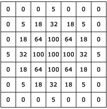
Gaussian Blur:
Below is a Gaussian Kernel (source)
logo_gauss = cv2.GaussianBlur(logo, (5,5), 0)
plt.rcParams["figure.figsize"] = (10,3)
plt.imshow(logo_gauss)
<matplotlib.image.AxesImage at 0x7f3c1ef35198>

-
Median Filtering:
Computes the median of all the pixels under the kernel window & the central pixel is replaced by the median value. Highly effective in removing salt-and-pepper noise.
We’ll first download an image having salt-and-pepper noise:
!curl "https://upload.wikimedia.org/wikipedia/commons/f/f4/Noise_salt_and_pepper.png" > sp.png
  % Total    % Received % Xferd  Average Speed   Time    Time     Time  Current
                                 Dload  Upload   Total   Spent    Left  Speed
100 82829  100 82829    0     0  39024      0  0:00:02  0:00:02 --:--:-- 51703
sp = cv2.imread('sp.png')
sp_median = cv2.medianBlur(sp,5)

plt.rcParams["figure.figsize"] = (20,7)
plt.subplot(1,2,1),plt.imshow(sp),plt.title('Salt & Pepper')
plt.xticks([]), plt.yticks([])
plt.subplot(1,2,2),plt.imshow(sp_median),plt.title('Processed')
plt.xticks([]), plt.yticks([])
plt.tight_layout()
plt.show()

-
Bilateral Filtering:
The previous 2 approaches remove the noise as well as the edges. Bilateral Filtering does the noise removal, but it keeps the edges. We’ll compare the three images (with noise, Gaussian & Bilateral) side by side, to check the differences.
Downloading the image:
!curl "https://upload.wikimedia.org/wikipedia/commons/d/d2/512x512-Gaussian-Noise.jpg" > gauss.jpg
  % Total    % Received % Xferd  Average Speed   Time    Time     Time  Current
                                 Dload  Upload   Total   Spent    Left  Speed
100 94314  100 94314    0     0  50518      0  0:00:01  0:00:01 --:--:-- 65541
gauss = cv2.imread('gauss.jpg')
gauss_gauss = cv2.GaussianBlur(gauss, (5,5), 0)

#bilateralFilter(input array (image), output array, diameter of pixel neighbour hood, sigmaColor, sigmaSpace)
gauss_bilateral = cv2.bilateralFilter(gauss, 9, 75, 75)
plt.rcParams["figure.figsize"] = (15,6)
plt.subplot(1,3,1), plt.imshow(gauss),plt.title('Original with noise')
plt.xticks([]), plt.yticks([])
plt.subplot(1,3,2), plt.imshow(gauss_gauss),plt.title('Gaussian Filter')
plt.xticks([]), plt.yticks([])
plt.subplot(1,3,3), plt.imshow(gauss_bilateral),plt.title('Bilateral Filter')
plt.xticks([]), plt.yticks([])
plt.show()

As you ca see, the Bilateral Filter doesn’t have hazy edges like the Gaussian.
Morphological Transformation
Morphological Transformations are basically playing with the shape of the original image, manipulating the internals of the image. There are 2 major operations: Erosion & Dilation.
-
Erosion:
Similar to the erosion of banks of a river, we try to erode away boundaries of the foreground object.

The kernel slides through the image (as in 2D convolution). A pixel in the original image (either 1 or 0) will be considered 1 only if all the pixels under the kernel is 1, otherwise it is eroded (made to zero). It is advisable to have the foreground as white (for reasons above).
!curl "http://pad1.whstatic.com/images/thumb/e/ef/Divide-Double-Digits-Step-9-Version-5.jpg/aid281771-v4-728px-Divide-Double-Digits-Step-9-Version-5.jpg" > digits.png
  % Total    % Received % Xferd  Average Speed   Time    Time     Time  Current
                                 Dload  Upload   Total   Spent    Left  Speed
100 46846  100 46846    0     0  48692      0 --:--:-- --:--:-- --:--:-- 50644
digits = cv2.imread('digits.png')
plt.imshow(digits)
<matplotlib.image.AxesImage at 0x7f3c1ee0c748>

digits = cv2.cvtColor(digits, cv2.COLOR_BGR2GRAY)
plt.imshow(digits, cmap=plt.get_cmap('gray'))
<matplotlib.image.AxesImage at 0x7f3c1ed45898>

ret, mask = cv2.threshold(digits, 200, 255, cv2.THRESH_BINARY_INV)
plt.imshow(mask, cmap='gray')
<matplotlib.image.AxesImage at 0x7f3c1ee77fd0>

kernel = np.ones((5,5), np.uint8)
eroded = cv2.erode(mask, kernel, iterations=1)
plt.imshow(eroded, cmap='gray')
<matplotlib.image.AxesImage at 0x7f3c1edce4a8>

-
Dilation:
You just make it fat! Remember the phrase, “Dilation of Pupil”.

kernel = np.ones((5,5), np.uint8)
dilated = cv2.dilate(mask, kernel, iterations=1)
plt.imshow(dilated, cmap='gray')
<matplotlib.image.AxesImage at 0x7f3c1ecf5cc0>

-
Opening & Closing:
Opening is just another name of erosion followed by dilation. It is useful in removing noise.
Closing is reverse of Opening, Dilation followed by Erosion. It is useful in closing small holes inside the foreground objects, or small black points on the object.
How do we remove noise? If we have white holes in the object as below:
ret, mask = cv2.threshold(sp, 100, 255, cv2.THRESH_BINARY)
plt.imshow(mask, cmap='gray')
<matplotlib.image.AxesImage at 0x7f3c1ec670b8>

We’ll apply Opening to the image.
opening = cv2.morphologyEx(mask, cv2.MORPH_OPEN, kernel)
plt.imshow(opening, cmap='gray')
<matplotlib.image.AxesImage at 0x7f3c1ebdb4e0>

As we can see above, there were still black dots inside the image that weren’t taken care of. We’ll do that using Closing
closing = cv2.morphologyEx(opening, cv2.MORPH_CLOSE, kernel)
plt.imshow(closing, cmap='gray')
<matplotlib.image.AxesImage at 0x7f3c1eb4d940>

The final outcome is disastrous, but you get the point right! Next in line is Morphological Gradient.
-
Morphological Gradient
Difference between dilation & erosion of an image.
ret, mask = cv2.threshold(digits, 200, 255, cv2.THRESH_BINARY_INV)
kernel = np.ones((3,3), np.uint8)
gradient = cv2.morphologyEx(mask, cv2.MORPH_GRADIENT, kernel)

plt.subplot(1,2,1), plt.imshow(mask, cmap='gray'),plt.title('Original')
plt.xticks([]), plt.yticks([])
plt.subplot(1,2,2), plt.imshow(gradient, cmap='gray'),plt.title('Morphological Gradient')
plt.xticks([]), plt.yticks([])
plt.show()

Image Gradients

Image gradients can be used to extract information from images. Gradient images are created from the original image (generally by convolving with a filter, one of the simplest being the Sobel filter) for this purpose. Each pixel of a gradient image measures the change in intensity of that same point in the original image, in a given direction. To get the full range of direction, gradient images in the x and y directions are computed.
One of the most common uses is in edge detection. One example of an edge detection algorithm that uses gradients is the Canny edge detector.
Consider the image, receipt, which we used previously.
plt.rcParams["figure.figsize"] = (20,10)
plt.imshow(receipt, cmap='gray')
<matplotlib.image.AxesImage at 0x7f3c1ea76c18>

1. Sobel & Scharr Derivatives
$\textbf{Sobel Operators = Gaussian Smooting + Differentiation Operator}$
In the image at the start of this topic, we can see the directions. These directions are specified by the yorder & xorder (vertical & horizontal respectively).
Size of the kernel, ksize can be specified (any value, generally if ksize=5 the kernel is 5x5).
If ksize=-1, a Scharr filter is used (?)
2. Laplacian Derivatives
Laplacian of the image is given by: $\Delta src = \frac{\partial ^2{src}}{\partial x^2} + \frac{\partial ^2{src}}{\partial y^2}$
Each derivative is found using Sobel derivatives.
plt.rcParams["figure.figsize"] = (20,10)
plt.imshow(receipt,cmap = 'gray')
plt.title('Original'), plt.xticks([]), plt.yticks([])
(<matplotlib.text.Text at 0x7f3c1e9b8ba8>,
 ([], <a list of 0 Text xticklabel objects>),
 ([], <a list of 0 Text yticklabel objects>))

sobelx = cv2.Sobel(receipt, cv2.CV_8U, 1, 0, ksize=3)
plt.rcParams["figure.figsize"] = (20,10)
plt.imshow(sobelx, cmap='gray')
plt.show()

sobely = cv2.Sobel(receipt, cv2.CV_16U, 0, 1, ksize=5)
plt.rcParams["figure.figsize"] = (20,10)
plt.imshow(sobely, cmap='gray')
plt.show()

scharrx = cv2.Sobel(receipt, cv2.CV_16U, 1, 0, ksize=-1)
plt.rcParams["figure.figsize"] = (20,10)
plt.imshow(scharrx, cmap='gray')
plt.show()

scharry = cv2.Sobel(receipt, cv2.CV_16U, 0, 1, ksize=-1)
plt.rcParams["figure.figsize"] = (20,10)
plt.imshow(scharry, cmap='gray')
plt.show()

laplacian = cv2.Laplacian(receipt, cv2.CV_8U)
plt.rcParams["figure.figsize"] = (20,10)
plt.imshow(laplacian, cmap='gray')
plt.show()

Canny Edge Detection
Canny Edge Detection is a popular edge detection algorithm. It was developed by John F. Canny in 1986. It is a multi-stage algorithm.
It goes through the following stages:
-
Noise Reduction:
Edge detection, as in the previous few topics, we know that it is succeptible to noise. Canny Edge detector takes care of that.
-
Finding Intensity Gradient of the Image.
The image is then passed through Sobel filter, both in horizontal & vertical direction.
-
Non-maximum suppression
(Difficult to explain)
-
Hysteresis Thresholding
This stage decides which are edges and which are not. This also removes small pixel noises on the assumption that the edges are along the lines.
edge_receipt = cv2.Canny(receipt, 150, 300)
plt.imshow(edge_receipt, cmap='gray')
plt.show()

Probably, not a great image to do edge detection. Let’s look at detecting road lanes.
!curl "http://www.richmondregional.org/images/monthly_flyer/September_2010_Graphics/DTE_ORT_lanes.jpg" > road_lanes.jpg
  % Total    % Received % Xferd  Average Speed   Time    Time     Time  Current
                                 Dload  Upload   Total   Spent    Left  Speed
100  496k  100  496k    0     0  78521      0  0:00:06  0:00:06 --:--:--  127k
road_lanes = cv2.imread('road_lanes.jpg')
road_lanes = cv2.cvtColor(road_lanes, cv2.COLOR_BGR2GRAY)
plt.imshow(road_lanes, cmap='gray')
<matplotlib.image.AxesImage at 0x7f3c1e88a6a0>

road_canny = cv2.Canny(road_lanes, 100,200)
plt.rcParams['figure.figsize'] = (15,7)
plt.imshow(road_canny, cmap='gray')
plt.show()

Contours
Contours by definition: An outline representing or bounding the shape or form of something.
In the above road lane detection, we got the threholded image. To create a boundary around it, we need the help of contours. More reading
!curl "https://www.echalk.co.uk/amusements/Games/Tetrominoes/shareIcons/shareIcon.jpg" > tetris.jpg
  % Total    % Received % Xferd  Average Speed   Time    Time     Time  Current
                                 Dload  Upload   Total   Spent    Left  Speed
100 30401  100 30401    0     0  17879      0  0:00:01  0:00:01 --:--:-- 19740
tetris = cv2.imread('tetris.jpg')
tetris_gray = cv2.cvtColor(tetris, cv2.COLOR_BGR2GRAY)
ret, mask = cv2.threshold(tetris_gray, 200, 255, cv2.THRESH_BINARY_INV)
plt.imshow(mask, cmap='gray')
<matplotlib.image.AxesImage at 0x7f3c1eb1a470>

We’ll get the blue blocks, for that we need to use cv2.inRange()
tetris_color = cv2.cvtColor(tetris, cv2.COLOR_BGR2RGB)
blue_lower = np.array([50, 0, 0], dtype='uint8')
blue_upper = np.array([255, 0, 0], dtype='uint8')
mask_blue = cv2.inRange(tetris_color, blue_lower, blue_upper)
plt.imshow(mask_blue)
<matplotlib.image.AxesImage at 0x7f3c1e790710>

output = cv2.bitwise_and(tetris_color, tetris_color, mask = mask_blue)
plt.imshow(output)
<matplotlib.image.AxesImage at 0x7f3c1e779e80>

output = cv2.cvtColor(output, cv2.COLOR_BGR2RGB)
plt.imshow(output)
<matplotlib.image.AxesImage at 0x7f3c1e6e84e0>

output_gray = cv2.cvtColor(output, cv2.COLOR_RGB2GRAY)
plt.imshow(output_gray, cmap='gray')
<matplotlib.image.AxesImage at 0x7f3c1e651b00>

_, contours, hierarchy = cv2.findContours(output_gray.copy(), cv2.RETR_LIST, cv2.CHAIN_APPROX_SIMPLE)
cont_digits = cv2.drawContours(output.copy(), contours, -1, (0, 255, 0), 3)
plt.imshow(cont_digits, cmap='gray')
plt.show()

Contour Features
In statistics, Moments are the quantitative measures to define data points. The moments defined are:
- Total Probability (Zeroth moment)
- Mean (1st moment)
- Variance (2nd moment)
- Skewness (3rd moment)
- Kurtosis (4th moment)
Image moments helps us to create features: center of mass of object, area of the object.
We already have to contours from the above image, calculating the moments.
!curl "http://vignette3.wikia.nocookie.net/marvel_dc/images/d/df/Flash_Logo_01.png/revision/latest?cb=20140529051349" > flash.png
  % Total    % Received % Xferd  Average Speed   Time    Time     Time  Current
                                 Dload  Upload   Total   Spent    Left  Speed
100  143k  100  143k    0     0   148k      0 --:--:-- --:--:-- --:--:--  161k
flash = cv2.imread('flash.png')
flash = cv2.cvtColor(flash, cv2.COLOR_BGR2RGB)
plt.imshow(flash)
<matplotlib.image.AxesImage at 0x7f3c1e5ad7b8>

flash_gray = cv2.cvtColor(flash, cv2.COLOR_RGB2GRAY)
ret, mask = cv2.threshold(flash_gray, 150, 255, cv2.THRESH_BINARY_INV)
plt.imshow(mask, cmap='gray')
<matplotlib.image.AxesImage at 0x7f3c1e526080>

_, contours, hierarchy = cv2.findContours(mask.copy(), cv2.RETR_LIST, cv2.CHAIN_APPROX_SIMPLE)
cont_flash = cv2.drawContours(flash.copy(), contours[6], -1, (0, 255, 0), 3)
plt.imshow(cont_flash, cmap='gray')
<matplotlib.image.AxesImage at 0x7f3c1e49a5c0>

NOTE: The official documentation as well as the popular blogs do not mention this regarding the contours. You need to find the specific contours for the shape in the image. So our flash contour would have a separate set of values here, likewise the circle inside which the flash sign is.
This is true everywhere, there will be situations where there are more than 100 contour values. God bless us then!
len(contours)
10
cnt = contours[6]
moments = cv2.moments(cnt)
print(moments)
{'nu11': -0.1907517670263885, 'nu30': -0.016394871693779282, 'nu03': 0.01208933681388529, 'mu30': -172121780.97688293, 'm01': 2010266.8333333333, 'nu21': 0.020979023957747672, 'mu02': 34511693.70050317, 'nu20': 0.1388066996783884, 'mu20': 14431539.936564565, 'mu21': 220248565.17384815, 'm10': 2147855.6666666665, 'nu12': -0.02132463374655408, 'm21': 83909645927.7, 'mu12': -223876954.18984604, 'mu11': -19832196.50196892, 'm12': 82711294309.23334, 'm00': 10196.5, 'm02': 430841095.0833333, 'm30': 104252150772.20001, 'm11': 403623205.7916666, 'mu03': 126920065.13383484, 'nu02': 0.33194339092953673, 'm20': 466869529.9166666, 'm03': 98676519466.85}
#To find centroid:
cx = int(moments['m10']/moments['m00'])
cy = int(moments['m01']/moments['m00'])
print("The centroid is ({},{})".format(cx,cy))
The centroid is (210,197)
print("The contour area is {}".format(moments['m00']))
The contour area is 10196.5
We can find the contour area using cv2.contourArea()
print("The contour area is {}".format(cv2.contourArea(cnt)))
The contour area is 10196.5
# Finding the contour perimeter
perimeter = cv2.arcLength(cnt, True)
print(perimeter)
947.6336801052094
- Contour Approximation
approx = cv2.approxPolyDP(cnt, perimeter, True)
print(approx)
[[[301 52]]]
-
Bounding Rectangles
Selecting the bounding box only for the flash!
x, y, w, h = cv2.boundingRect(cnt)
rect = cv2.rectangle(flash.copy(), (x,y), (x+w, y+h), (0,255,0), 5)
plt.imshow(rect)
<matplotlib.image.AxesImage at 0x7f3c1e41c6d8>

rect = cv2.minAreaRect(cnt)
box = cv2.boxPoints(rect)
box = np.int0(box)
rect_draw = cv2.drawContours(flash.copy(), [box], 0, (255,0,0), 5)
plt.imshow(rect_draw, cmap='gray')
<matplotlib.image.AxesImage at 0x7f3c1e389cf8>

-
Minimum Enclosing Circle
Cover the ‘flash’ sign using a circle.
(x, y), radius = cv2.minEnclosingCircle(cnt)
center = (int(x), int(y))
radius = int(radius)
circle_draw = cv2.circle(flash.copy(), center, radius, (0,255,0), 4)
plt.imshow(circle_draw)
<matplotlib.image.AxesImage at 0x7f3c1e308828>

-
Fitting an Ellipse
To fit an ellipse to the flash sign.
ellipse = cv2.fitEllipse(cnt)
draw_ellipse = cv2.ellipse(flash.copy(), ellipse, (0,255,0), 4)
plt.imshow(draw_ellipse)
<matplotlib.image.AxesImage at 0x7f3c1e677048>

Histograms
A histogram represents the distribution of colors in an image. It can be visualized as a graph (or plot) that gives a high-level intuition of the intensity (pixel value) distribution. We are going to assume a RGB color space in this example, so these pixel values will be in the range of 0 to 255.
By looking at the histogram of an image, you get intuition about contrast, brightness, intensity distribution etc of that image.
!curl "https://media1.britannica.com/eb-media/54/155954-004-4BF4BBF7.jpg" > everest.jpg
  % Total    % Received % Xferd  Average Speed   Time    Time     Time  Current
                                 Dload  Upload   Total   Spent    Left  Speed
100 29947  100 29947    0     0  59170      0 --:--:-- --:--:-- --:--:--  117k
everest = cv2.imread('everest.jpg')
everest_gray = cv2.cvtColor(everest, cv2.COLOR_BGR2GRAY)
plt.imshow(everest_gray, cmap='gray')
<matplotlib.image.AxesImage at 0x7f3c1eb7f630>

- Plot histograms using just matplotlib
plt.hist(everest_gray.ravel(), 265, [0,256])
plt.show()

color = ('b', 'g', 'r')
for i, col in enumerate(color):
    histr = cv2.calcHist([everest], [i], None, [256], [0,256])
    plt.plot(histr, color=col)
    plt.xlim([0,256])

plt.show()

- Multi-Dimensional Histograms
hsv = cv2.cvtColor(everest, cv2.COLOR_BGR2HSV)
plt.imshow(hsv)
<matplotlib.image.AxesImage at 0x7f3c1df17e48>

# calcHist(images, channels, mask, histSize, ranges[, hist[, accumulate]])
hist = cv2.calcHist([hsv], [0,1], None, [180, 256], [0, 180, 0, 256])
plt.imshow(hist, interpolation='nearest')
<matplotlib.image.AxesImage at 0x7f3c1df033c8>

Applications of histograms still feels as something very obscure at this point of time. Let’s continue the discussion after I understand things.
This should get you started off with using OpenCV at a very primary level. Even I’ve not mastered it, still to cover a lot of ground. Next part would be using all the learnings to create an application or maybe a Kaggle competition dataset for practice.